
Of course, I would have to use parametric equations to achieve this. My first concern was the proper spacing of t. I decided to use "contact points" at what appeared to be the extrema of my graph. I counted 5 such points on the way up and 5 on the way down. It wasn't hard to tell there would be some trig functions involved, so I worked with intervals of π. In total, each period of my curve would be of length t = 10π.

I had to create a y(t) that would move from –6 to 6 and back over the domain 0 < t < 10π. I could have used trig for this, but I wasn't brave enough to try to figure out how x and y interacted with each other. So instead I just gave y a constant rate of change and aimed for a triangle wave.
The basis for this would be the modulo function; in this case, we want y to restart at every interval of 5π, with appropriate scaling and positioning:


Of course, we want every other period of the function to slop downward, so we multiply by

to create our final y(t):

The function x(t) is quite a bit more difficult to design. I began by hand-drawing a curve that touches the "contact points" (the x-axis is in units of π):

Note that unlike y(t), which had a period of 10π, x(t) seems to have a period of only 5π (ignoring the gain in elevation).
The only way I could think of creating this function was to make it continuous but piecewise. In the domain π < t < 4π (mod 5π) we have what looks like a simple negative cosine wave. In the rest of the domain, we have... something else.

Let's worry about the cosine segment first. This:

would work just fine to model this part of the domain but for two problems. First, since x(t) has an odd periodicity in terms of π, we'll want the curve to "restart" every 5π. We'll do this by working with

in place of t:

Second problem: we'll need "damp down" the curve from 0 to π and again from 4π to 5π. We do this by multiplying by the following floor function a(t), itself a function of z(t):

This is the product of functions:

Now we have to fill in the gaps. After some experimentation, I concluded the best fit for my sketch was an arctan function. Once again, we use z(t) in place of t to establish periodicity, and multiply by 1 – a(t) to keep the function restricted to its proper domain:

One more step before simply adding the two functions together, and that's to add another floor function the mix:

This is to ensure that the "baseline elevation" increases by 1 every 5π.
Adding these three components, we have our final x(t)

which is continuous and hits the "contact points" as desired:

When we finally combine x(t) and y(t), what we get is one beautiful parametric graph:
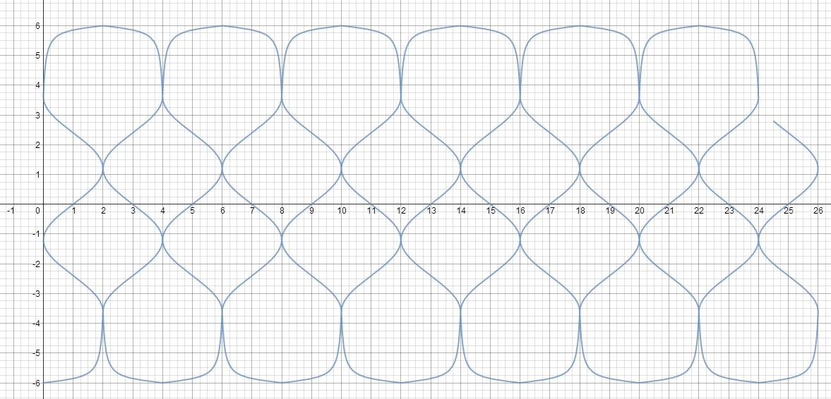
It looks pretty close to what I drew, right?
Here's the link on Desmos: https://www.desmos.com/calculator/tkdymhskxr
No comments:
Post a Comment